4. Control Synthesis with A/G Contract¶

PyCASSE enables reasoning about the behavior of a component \(M\), with given dynamics, using A/G contracts. In this chapter, we sythesize the control trajectory of a component with linear dynamics such that it implements a contract \(C\), i.e., \(M \models C\).

4.1. Control Synthesis with STL A/G Contract in PyCASSE¶

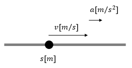
Assume a point-mass robot on a line where its location, velocity, and acceleration are denoted as \(s\), \(v\), and \(a\).

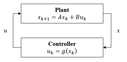
The dynamics of the point-mass robot \(M\) on a line is given as \(x_{k+1} = A x_k + B u_k\) where \(x_k = [s_k, v_k]^T\) and \(u_k = [a_k]\). The goal is to synthesize the control input \(\mathbf{u}^{15} = u_0 u_1 \ldots u_{14}\) where \(\forall k, u_k \in [-1, 1]\) such that the robot visits the regions \(\{ r | r \geq 3\}\) and \(\{ r | r \leq 0\}\) every \(5~s\), i.e., \(\phi_G := \mathbf{G}_{[0,10]} ((\mathbf{F}_{[0,5]} (s \geq 3)) \land (\mathbf{F}_{[0,5]} (s \leq 0)))\) is satisfied.

Given the initial state \(x_0 = [0, 0]^T\), PyCASSE can synthesize the control input by running the following Python script:

from pycasse import *
import matplotlib.pyplot as plt
import time

# Build a contract
c = contract('c')                                               # Create a contract c
c.add_deter_vars(['s', 'v', 'a'],
   bounds = [[-100, 1000], [-5, 10], [-1, 1]])                  # Set deterministic variables
c.set_assume('True')                                            # Set/define the assumptions
c.set_guaran('G[0,10] ((F[0,5] (s => 3)) & (F[0,5] (s <= 0)))') # Set/define the guarantees
c.saturate()                                                    # Saturate c
c.printInfo()                                                   # Print c

# Initialize a milp solver and add a contract
solver = MILPSolver()
solver.add_contract(c)

# Build a linear system dynamics
solver.add_dynamics(x = ['s', 'v'], u = ['a'], A = [[1, 1], [0, 1]], B = [[0], [1]])

# Add initial conditions
solver.add_init_condition('s == 0')
solver.add_init_condition('v == 0')

# Add guarantee constraints
solver.add_constraint(c.guarantee, name='b_g')

# Solve the problem using MILP solver
start = time.time()
solved = solver.solve()
end = time.time()
print("Time elaspsed for MILP: {} [seconds].\n".format(end - start))

# Print and plot the trajectory of the component/system
if solved:
   # Print the trajectory
   comp_traj = solver.print_solution()

   # Plot the trajectory
   fig, axs = plt.subplots(1,3)
   fig.set_figwidth(20)
   fig.set_figheight(5)
   x = list(range(16))
   thres1 = [3]*16
   thres2 = [0]*16
   axs[0].plot(x, comp_traj['s'])
   axs[0].plot(x, thres1, 'r')
   axs[0].plot(x, thres2, 'r')
   axs[0].set_xlabel(r'$Time [s]$', fontsize='large')
   axs[0].set_ylabel(r'$s [m]$', fontsize='large')

   axs[1].plot(x, comp_traj['v'])
   axs[1].set_xlabel(r'$Time [s]$', fontsize='large')
   axs[1].set_ylabel(r'$v [m/s]$', fontsize='large')

   axs[2].plot(x, comp_traj['a'])
   axs[2].set_xlabel(r'$Time [s]$', fontsize='large')
   axs[2].set_ylabel(r'$a [m/s^2]$', fontsize='large')

   # Save the figure
   plt.savefig('test_dyn_stl_log_fig.pdf')

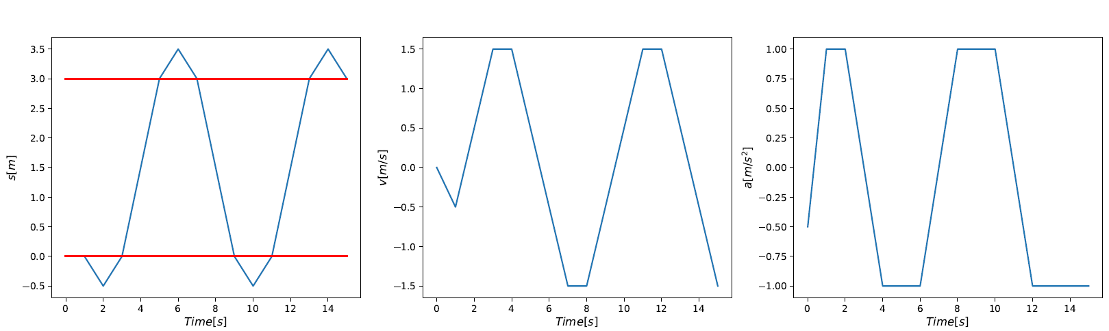
The figure on the left shows the trajectory of the robot’s location; the figure on the center shows the trajectory of the robot’s velocity; and the figure on the right shows the trajectory of the robot’s acceleration (control input). As shown in the above figure, the control input synthesized by PyCASSE guarantees the satisfaction of the STL specification \(\phi_G\).

For details, refer to test_dyn_stl.py.

4.2. Control Synthesis with StSTL A/G Contract in PyCASSE¶

Let’s assume the same point-mass robot on a line from the previous example, but this time, its plant is subject to Gaussian uncertainty \(w \sim Gaussin([0, 0]^T, [[0, 0], [0, 0.5^2]])\).

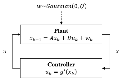
The dynamics of the point-mass robot \(M'\) on a line is given as \(x_{k+1} = A x_k + B u_k + w_k\) where \(x_k = [s_k, v_k]^T\) and \(u_k = [a_k]\). The goal is to synthesize the control input \(\mathbf{u}^{10} = u_0 u_1 \ldots u_9\) where \(\forall k, u_k \in [-1, 1]\) such that the robot eventually in \(10~s\) reaches the region \(\{ r | r \geq 34\}\) with probability larger than or equal to \(0.9\), i.e., \(\phi'_G := \mathbf{F}_{[0,10]} (\mathbb{P} \{ s \geq 34 \} \geq 0.9)\) is satisfied.

Given the initial state \(x_0 = [0, 0]^T\), PyCASSE can synthesize the control input by running the following Python script:

from pycasse import *
import matplotlib.pyplot as plt
import time

# Build a contract
c_prime = contract('c_prime')                    # Create a contract c_prime
c_prime.add_deter_vars(['s', 'v', 'a'],
   bounds = [[-100, 2000], [-5, 10], [-1, 1]])   # Set deterministic variables
c_prime.set_assume('True')                       # Set/define the assumptions
c_prime.set_guaran('F[0,10] (P[0.9] (s => 34))') # Set/define the guarantees
c_prime.saturate()                               # Saturate c_prime
c_prime.printInfo()                              # Print c_prime

# Initialize a milp solver and add a contract
solver = MILPSolver()
solver.add_contract(c_prime)

# Build a linear system dynamics
solver.add_dynamics(x = ['s', 'v'], u = ['a'], A = [[1, 1], [0, 1]], B = [[0], [1]], Q = [[0, 0], [0, 0.5**2]])

# Add initial conditions
solver.add_init_condition('s == 0')
solver.add_init_condition('v == 0')

# Add guarantee constraints
solver.add_constraint(c_prime.guarantee, name='b_g')

# Solve the problem using MILP solver
start = time.time()
solved = solver.solve()
end = time.time()
print("Time elaspsed for MILP: {} [seconds].\n".format(end - start))

# Print and plot the trajectory of the component/system
if solved:
   # Print the trajectory
   comp_traj = solver.print_solution()

   # Plot the trajectory
   fig, ax = plt.subplots()
   x = list(range(11))

   ax.plot(x, comp_traj['a'])
   ax.set_xlabel(r'$Time [s]$', fontsize='large')
   ax.set_ylabel(r'$a [m/s^2]$', fontsize='large')

   # Save the figure
   plt.savefig('test_dyn_ststl_log_fig.pdf')

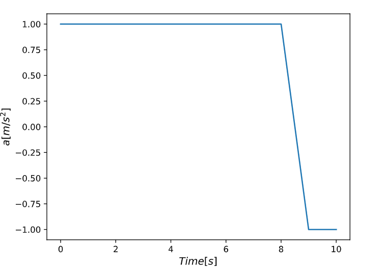
The above figure shows the trajectory of the robot’s acceleration (control input) synthesized by PyCASSE. To validate whether the the synthesized control input satisfies the StSTL specification \(\phi'_G\), \(10^5\) MATLAB simulations were ran by using the synthesized control input.

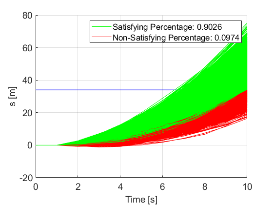
\(10^5\) simulation in MATLAB.

As shown in the simulation results, the control input synthesized by PyCASSE satisfies the StSTL specification \(\phi'_G\). For details, refer to test_dyn_ststl.py and test_dyn_ststl_simu.m.

4.3. PyCASSE MILPSolver Class¶

class pycasse.MILPSolver(mode='Boolean', verbose=False)¶

A contract class for defining a mip solver.

add_constraint(node, hard=True, name='b')¶

Adds contraints of a STL/ StSTL formula to the MIP solver.

Parameters:	node (`pycasse.ASTObject`) – An abstract syntax tree (AST) object representing an STL or an StSTL formula hard (bool, optional) – If False, add soft constraints, defaults to True where hard constraints are added name (str, optional) – The name of the Boolean variable tied to the STL/StSTL formula, defaults to b

add_contract(contract)¶

Adds a contract to the MILP solver.

Parameters:	contract (`pycasse.contracts.contract`) – A contract object.

add_dynamics(x=[], u=[], z=[], A=None, B=None, C=None, D=None, E=None, Q=None, R=None)¶

Adds constraints for dynamics of the system (or a component). x_{k+1} = A*x_{k} + B*u_{k} + w_{k} z_{k} = C*x_{k} + v_{k} u_{k} = D*z_{k} + E

Parameters:

x (list, optional) – A list of str representing the state of the system, defaults to []
u (list, optional) – A list of str representing the control input of the system, defaults to []
z (list, optional) – A list of str representing the measurement of the system, defaults to []
A (list[list[float]], optional) – A matrix representing process of the system, defaults to None
B (list[list[float]], optional) – A matrix representing process of the system, defaults to None
C (list[list[float]], optional) – A matrix representing measurements of the state of the system, defaults to None
D (list[list[float]], optional) – A matrix deciding the control input of the system, defaults to None
E (list[list[float]], optional) – A matrix deciding the control input of the system, defaults to None
Q (list[list[float]], optional) – A covariance matrix representing the process error of the system, defaults to None
R (list[list[float]], optional) – A covariance matrix representing the measurement error of the system, defaults to None

add_init_condition(formula)¶

Adds constraints for an initial condition.

Parameters:	formula (str) – An StSTL or a STL formula.

print_solution(node_var_print=False)¶

Prints the solution of the MIP.

Parameters:	node_var_print (bool, optional) – If True prints the solution of the MIP solver, defaults to False
Returns:	A dictionary of the trajectories of the deterministic variables
Return type:	dict

solve()¶: Solves the MIP problem.