6. Examples
All the exampels are located in the examples folder.
- contract_tests contains examples which checks contract compatibility, consistency, and feasibility, along with composition/ conjunction of multiple contracts, and refinements relationship between two contracts.
- stl_tests contains examples where STL is utilized to specify A/G contracts.
- ststl_test contains examples where StSTL is utilized to specify A/G contracts.
- parametric_tests contains examples where parameters are synthesized.
- ICCAD2022 contains case studies for the paper [Oh22] published at ICCAD 2022.
6.1. Parameter Synthesis using StSTL Contracts (ICCAD 2022)
6.1.1. Finding Parameters for Multi-Sensor Perception system
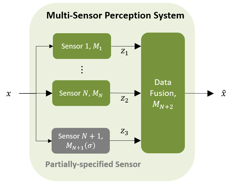
Assume a multi-sensor perception system with \(N\) fully specified sensors and \(L\) partially specified sensors captured by parametric stochastic contracts.
In this case study, we aim to search for inexpensive sensors that can be affected by noise, i.e., large standard deviations \(\sigma_j\) within the \([0.2, 2]\) range, while still guaranteeing with probability (confidence) \(p_j\) in \([0.8, 1]\) that the sensor error lies in the \([-1, 1]\) interval, where \(j = 1, \cdots, L\).
We assume that there exists only one unspecified sensor, i.e., \(L = 1\), and find the optimal set of parameters \(\left( p_{N+1}, \sigma_{N+1} \right)\) for the unspecified sensor such that the composition of the component-level contracts robustly refines the system-level contract, i.e., \(\bigotimes_{i=1}^{N} C_i \otimes C_{N+1} \otimes C_{N+2} \preceq_{\rho^*} C_{per}\) and \(M_{N+1} ( \sigma_{N+1} ) \models_{\rho^*} C ( p_{N+1} )\).
The case study can be run:
$ python3 examples/ICCAD2022/sensor_experiment.py
As a result, feasible regions for finding the set of optimal parameter values \(\pi_{safe} = (c_s, p_s)\) when there exists a single fully specified sensor, i.e., \(N=1\), is :
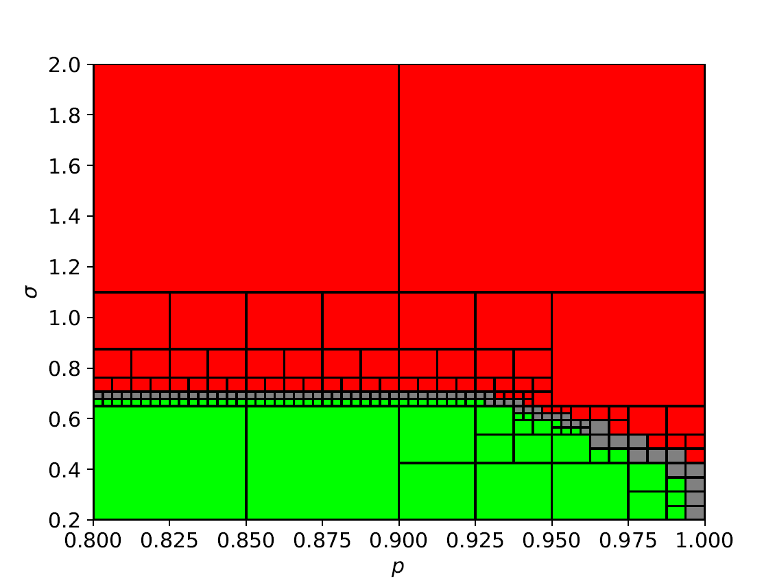
and given the cost function \(J(p_{2}, \sigma_2) = - p_{2} - 10 \sigma_{2}\), the optimal paramter values is \((p_{2}^*, \sigma_{2}^*) = (0.9281, 0.6781)\).
Feasible regions for finding the set of optimal parameter values \(\pi_{safe} = (c_s, p_s)\) when there exists three fully specified sensors, i.e., \(N=3\), is :

and given the cost function \(J(p_{4}, \sigma_4) = - p_{4} - 10 \sigma_{4}\), the optimal paramter values is \((p_{4}^*, \sigma_{4}^*) = (0.8063, 1.1563)\).
6.1.2. Finding Parameters for Cruise Control System
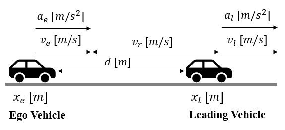
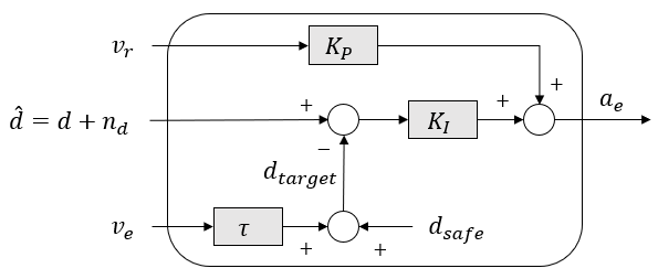
The cruise control system in the figure above controls the ego vehicle to keep it as close as possible to a target distance \(d_{target} = d_{safe} + \tau v_e\), while adapting to the leading vehicle’s behavior. \(d_{safe}\) is the pre-determined safe distance and \(\tau\) is the time gap. Several parts of such system are intrinsically of stochastic nature, e.g., the noise of the sensors detecting the distance and velocity, and the behavior of the leading vehicle. In this case study, we illustrate the parameter synthesis process on an system whose safety and comfort requirements are specified by two parametric stochastic contracts.
In this case study, we search for the sets of optimal parameter values \(\pi_{safe} = (c_s, p_s)\) and \(\pi_{comf} = (c_c, p_c)\) for two requirements expressed as the parametric stochastic contracts \(C_{safe}(\pi_{safe})\) and \(C_{comf}(\pi_{comf})\).
\(C_{safe}\) requires that the probability of maintaining the distance \(d\) larger than or equal to \(c_{s}\) is greater than or equal to \(p_{s}\) when the initial distance is greater than or equal to \(d_{target}\) and the initial relative velocity between the ego and the leading vehicle is smaller than or equal to \(5~m/s\).
\(C_{safe} = (\phi_{A,safe}, \phi_{G,safe})\) where \(\phi_{A,safe} := (d \geq d_{target}) \land (|v| \leq 5)\) and \(\phi_{G,safe} := \mathbf{G}_{[0,20]} ( c_{s} - d )^{[p_{s}]}\)
\(C_{comf}\) requires that the acceleration of the ego vehicle be larger than or equal to \(c_{c}~m/s^2\) with a probability larger than or equal to \(p_{c}\), to avoid abrupt decelerations under the same assumptions as \(C_{safe}\).
\(C_{comf} = (\phi_{A,comf}, \phi_{G,comf})\) where \(\phi_{A,comf} := (d \geq d_{target}) \land (|v| \leq 5)\) and \(\phi_{G,comf} := \mathbf{G}_{[0,20]} ( c_{c} - a_e ) ^{[p_{c}]}\)
The case study can be run:
$ python3 examples/ICCAD2022/ACC_experiment.py
As a result, feasible regions for finding the set of optimal parameter values \(\pi_{safe} = (c_s, p_s)\):
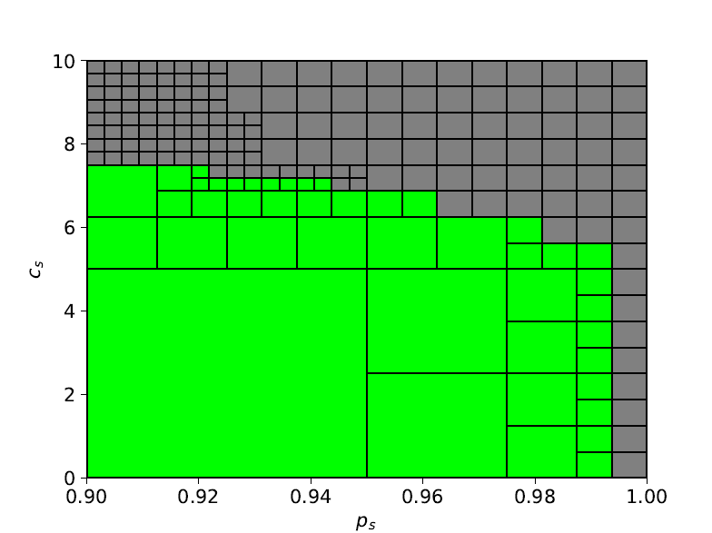
and the optimal paramter values is \((c_{s}^*, p_{s}^*) = (5.625, 0.99375)\).
Similarly, feasible regions for finding the set of optimal parameter values \(\pi_{comf} = (c_c, p_c)\) can be found:
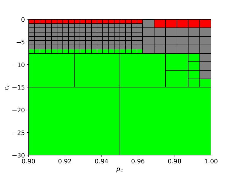
and the optimal paramter values is \((c_{c}^*, p_{c}^*) = (-7.5, 0.99375)\).